parse2wig: make wig files
Parse2wig converts a map file (SAM, BAM or Bowtie format) into chromosome-separated wig files.The generated wig files of each ChIP and Input sample will be used as input for drompa2.
Options
parse2wig2 -i inputfile -o output_prefix -gt genome_table

       file formats: -sam (default) / -bam (require samtools) / -bowtie
       -binsize: bin size (default: 100bp)
       -rcenter: consider bp around the center of fragment
       -odir: output directory name (default:parse2wig2dir)
       -of: output format (default: 0)
             0; binary file (.bin)
             1; compressed wig file (.wig.gz)
             2; uncompressed wig file (.wig)
For single-end file
       -flen: expected fragment length (default: 150bp)
For paired-end file
       -pair: add when the input file is paired-end
       -maxins: maximum fragment length (default: 500bp)

For normalization
       -norm: normalize type (default:1)
             0; not normlize
             1; normlize for whole genome
             2; normlize for each chromosome
       -num4rpkm: normalized mapped reads per 1M regions (default:10000)
       -makengc: make GCov data
       -win4gc: window size for genome coverage (default:10000)
       PCR bias:
             -nofilter: do not filter PCR bias
             -tf: PCRbias threshold (default: more than 1 reads)
       Mappability:
             -mp: normalization with mappability
             -mpsize: windowsize of mappability score (default: 1000bp)
             -mpthre: threshold of low mappability (default: 0.3)
       GC content: (require genome sequence, take large time and memory)
             -GC: read normalization based on GC content of reference genome
             -igpeak: for ignoring ChIP-peak regions for GC normalization:
             -GCref: (with -GC option) read normalization based on GC content of reference sample (require GCdist.xls, for comparison of multiple ChIP samples)
             -max4gc: max value for weights of GCdist (default: 10, specify 0 when threshold is not necessary)
Examples
For example, the command:% parse2wig2 -i ChIP.sam -o ChIP -gt genome_table-hg19.txt -binsize 100
makes wig files for ChIP.sam with bin size of 100 bp. The wig files for chromosomes are created in the directory ./(output directory)/ (default: parse2wig2dir).
The stats file "ChIP.100.xls" is also produced in the output directory, which describes the total read number, genome coverage, percentage of filtered reads etc.
Parse2wig can output wig files in binary (.bin), compressed (.wig.gz) and uncompressed (.wig) format with "-of" option.
Compressed wig files generated by parse2wig can be used for other visualizing programs and browser.
Mapped reads are extended to the expected DNA-fragment length (150 bp by default). The length of each read is calculated from the mapfile.
If using fragments with 200 bp long and you want to consider only around 50 bp around center of each fragment, type as below:
% parse2wig2 -i ChIP.sam -o ChIP -gt genome_table-hg19.txt -flen 200 -rcenter 50
When parsing BAM-formatted paired-end file, supply "-pair" option:
% parse2wig2 -bam -pair -i ChIP-paired.bam -o ChIP -gt genome_table-hg19.txtFor paired-end file, the length of each fragment is calculated from the mapfile.
The inter-chromosome read-pairs are rejected. Use "-maxins" option to change the maximum fragment length allowed.
Note: When the input mapfile is paired-end and bam-formatted, use NOT-SORTED bam because parse2wig2 uses the order of paired-end mapped reads.
Filtering reads
Parse2wig filters duplicated reads as "PCR bias" from map file (see reference in detail.) The proportion of filtered reads can be checked by output xls file.If filtering procedure is not necessary, supply "-nofilter" option:
% parse2wig2 -i ChIP.sam -o ChIP -gt genome_table-hg19.txt -nofilter
Normalization
Parse2wig normalizes the wig data with the number of total mapped reads (after filtering) for the comparison of multiple ChIP samples.By default, the number of each bin is normalized for whole-genome level (5,000 reads per 1M-bp of genome). This value can be changed by "-num4rpkm" option.
Other normalizations:
  % parse2wig2 -i ChIP.sam -o ChIP -gt genome_table-hg19.txt -norm0  # not normalize
  % parse2wig2 -i ChIP.sam -o ChIP -gt genome_table-hg19.txt -norm2  # normalize for each chromosome
Mappability
Parse2wig can normalize reads with genome-mappability by supplying mappability files as below:% parse2wig2 -i ChIP.sam -o ChIP -gt genome_table-hg19.txt -mp mpfiledir/50-n2-m1 -mpsize 1000
The appropriate mappability files depend on the parameters for genome-mapping. For the files of mappability data, see Mappability file section.
GC content
under constructionDROMPA: peak-calling
DROMPA has commands for peak-calling, read-distribution visualization and several other optional functions.Commands are as follows:
Usage: drompa2 command [options]

Command: PEAKCALL_P  peak-calling (Binomial test)
                PEAKCALL_W  peak-calling (Wilcoxon test)
                PEAKCALL_E  peak-calling (Enrichment ratio)
                GV                global-view visualization
                PD                peak density
                COUNTTAG    count total tags in bed regions specified
                CI                 compare peak-intensity between two samples
                GOVERLOOK  genome-wide overlook of peak positions
                PROFLE         make R script of averaged read density
Peak-calling with significant test
DROMPA has two types of significant test for peak-calling. One is PEAKCALL_P, the peak-calling strategy similar as PeakSeq, which adopts the Poisson test for ChIP-internal enrichment and Binomial test for ChIP/Input enrichment. Another is PEAKCALL_W, which adopts Wilcoxon-test for ChIP/Input enrichment, same as DROMPA1. We recommend PEAKCALL_P for the general peak-calling.Options (Input and Output)
       -sm : smoothing bin with N bp window (default: off)
       -binsize : bin size of wig files (default: 100)
       -bs: change bin size of Nst sample
       -optype: output type
            1: peak file and figure (default)
            2: figure only
            3: peak file only
            4: output enrichment profiles
       -norm: ChIP/Input normalization type
            0: not normalize
            1: with total read number (default)
            2: with NCIS method (normalize with background reads of ChIP sample, see [3])

       -mp: for normalization of mappability
       -mpsize: windowsize of mappability score (default: 1000bp)
       -mpthre: threshold of low mappability (default: 0.3)
       -outputYM: output peaks of chromosome Y and M (default: ignore)
       -if: 0;binary file, 1;compressed wig file (.wig.gz), 2;uncompressed wig file (.wig) (default: 0)
       -nosig: do not implement significant test (default: off)
Examples
% drompa2 PEAKCALL_P -i parse2wig2dir/ChIP -w parse2wig2dir/Input -p ChIP -optype3 -gt genome_table-hg19.txt
Then the peak-list file "ChIP.xls" is generated. This list is output in a tab-delimited text file that can be handled by a text editor or Microsoft Excel.
To change the thresholds for peak-calling, type for instance:
% drompa2 PEAKCALL_P -i parse2wig2dir/ChIP -w parse2wig2dir/Input -p ChIP -optype3 -gt genome_table-hg19.txt -pthre1 1e-4 -qthre 1 -ipm 20
If mappability file is supplied by "-mp" option, the low mappable regions (defined as "-mpthre") are ignored.
% drompa2 PEAKCALL_P -i parse2wig2dir/ChIP -w parse2wig2dir/Input -p ChIP -optype3 -gt genome_table-hg19.txt -mp mpfiledir/50-n2-m1 -mpsize 1000 -mpthre 0.25
Threshold
DROMPA has several thresholds for peak-calling.
       -pthre1 : p-value threshold for ChIP/Input enrichment
       -pthre2 : p-value threshold for ChIP internal
       -qthre : q-value threshold for ChIP/Input enrichment
       -ethre : IP/Input enrichment threshold
       -ipm : read intensity threshold of peak summit
P-value for "-pthre1" is estimated by binomial test for PEAKCALL_P and Wilcoxon test for PEAKCALL_W.
P-value for "-pthre2" is estimated by Poisson test for PEAKCALL_P and not used for PEAKCALL_W.
FDR (multiple hypothesis testing) is calculated by Benjamini-Hochberg method. This value strongly depends on the number of called peaks.
"-ethre" is not used in default for PEAKCALL_P and >3 in default for PEAKCALL_W. When analyzing "broad peaks" such as H3K36me3, it may be better to relax this threshold (e.g., >2).
"-ipm" is the threshold for IP reads in each peak summit which indicates "peak height".
We recommend the main threshold "-pthre1" or "-qthre" for PEAKCALL_P and "-ipm" for PEAKCALL_W.
DROMPA: visualization
DROMPA can visualize multiple ChIP samples with genome annotation specified.Options (for drawing)
- drawing parameter
       -png: output with png format (Note: output file is not merged)
       -LS: length per one line (kb) (default: 100kb)
       -LPP: number of lines per one page (default: 3)
       -chr: output only a chromosome specified
       -rmchr: remove chromosome-separated pdf file
       -r : specify the regions to visualize

       -show_ctag: display ChIPread lines (0:off 1:on)
       -show_itag: display Inputread lines (0:off 1:all 2:first one)
       -scale_tag : scale of read line
       -sct : scale of st read line
       -showratio: display enrichment ratio in liner scale (0: off, 1:liner, 2:log  default: 0)
       -scale_ratio : scale of ratio line
       -showpvalue1: display -log(pvalue) for ChIP internal
       -showpvalue2: display -log(pvalue) for ChIP/Input enrichment
       -scr : scale of st ratio line
       -bn : number of separations for y-axis (default: 2)
       -ystep : height of read line (default: 20)
       -g_ref : RefSeq gene list
       -g_ens : Ensembl gene list
       -g_scer : SGD annotation (S.cerevisiae)
       -g_spom : S.pombe gene list
       -ars : ARS list (for S.cerevisiae)
       -showars: display ARS only (do not display genes)
       -ter : TER list (for S.cerevisiae)
       -bed : specify the bedfile
       -bedname : specify the name of bedfile
       -repeat : Repeat list
       -graph : show graph such as GCcontents (default: none)
       -gcsize : resolution of GCcontents graph (default: 0)
Examples
Here we assume we have 4 ChIP samples (ChIP1, 2, 3 and 4) and one Input sample to be analyzed.The command
  % drompa2 PEAKCALL_P -p ChIPseq-hg19 -gt genome_table-hg19.txt \
  % -i parse2wig2dir/ChIP1-hg19 -w parse2wig2dir/Input-hg19 -name ChIP1 \
  % -i parse2wig2dir/ChIP2-hg19 -w parse2wig2dir/Input-hg19 -name ChIP2 \
  % -i parse2wig2dir/ChIP3-hg19 -w parse2wig2dir/Input-hg19 -name ChIP3 \
  % -i parse2wig2dir/ChIP4-hg19 -w parse2wig2dir/Input-hg19 -name ChIP4 \
  % -optype2 -g_ref refFlat_hg19.txt -LS1000 -LPP2 -scale_tag 50 -sct1 10
generates pdf files (chromosome-separated files and whole-genome file) with two lines per one page and 1-Mbp (1000-kbp) length for one line.
It is possible to change the scale of each read line (y-axis) with "-scale_tag" or "-sct" option.
This command can be rewritten as follows:
  % s1="-i parse2wig2dir/ChIP1-hg19 -w parse2wig2dir/Input-hg19 -name ChIP1"
  % s2="-i parse2wig2dir/ChIP2-hg19 -w parse2wig2dir/Input-hg19 -name ChIP2"
  % s3="-i parse2wig2dir/ChIP3-hg19 -w parse2wig2dir/Input-hg19 -name ChIP3"
  % s4="-i parse2wig2dir/ChIP4-hg19 -w parse2wig2dir/Input-hg19 -name ChIP4"
  % drompa2 PEAKCALL_P -p ChIPseq-hg19 -gt genome_table-hg19.txt $s1 $s2 $s3 $s4 -optype2 \
  % -g_ref refFlat_hg19.txt -LS1000 -LPP2 -scale_tag 50 -sct1 10
Hereafter we use "$s1 $s2 $s3 $s4" as ChIP samples.
In default, DROMPA visualize ChIP-read line only. You can show the lines of pvalue, enrichment, Input-read line as below (e.g., for yeast):
  % drompa2 PEAKCALL_P -p ChIPseq-yeast-all -gt genome_table-scer.txt $s1 -g_scer SGD_features.tab \
  % -optype2 -LS100 -showpvalue1 -showpvalue2 -showratio1 -show_itag2 -LPP2 -scale_tag 100 -scale_ratio 3 -sm 500
Figure sample 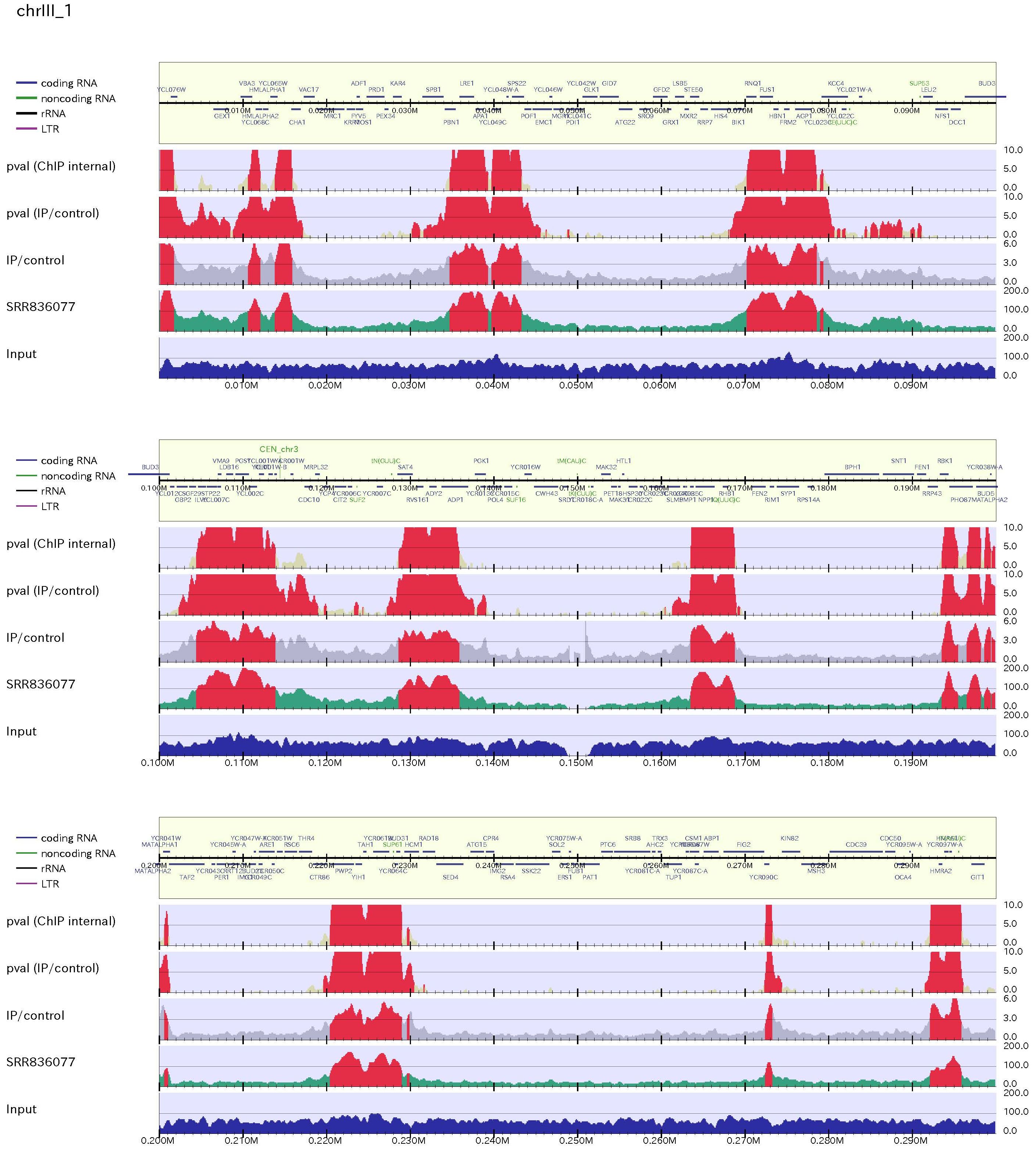
The green histogram indicates ChIP-read line and blue one does the Input-read line. the region which is above the threshold is highlighted in red. The red regions in ChIP-read line indicated peak regions.
If mappability file is supplied by "-mp" option, the low mappable regions (defined as "-mpthre") are shaded in the figure.
When "-chr" option specified, the figure of only specified chromosome is output. For example:
% drompa2 PEAKCALL_P -p ChIPseq-hg19 -gt genome_table-hg19.txt $s1 $s2 $s3 $s4 -optype2 -g_ref refFlat_hg19.txt -chr12This command output the result of chromosome 12 only.
Note: Chromosome number is identical with the order in the genome-table file. For instance, for human, generally chrX is after chr22, so supplying "-chr23" indicates showing chrX only.
To make the figure focusing some region (here MACF1 gene region), make "MACF1.txt", tab-separated region file and supply the option "-r MACF1.txt" as follows:
  % echo "chr1	39500000	40000000" > MACF1.txt
  % drompa2 PEAKCALL_P -g_ref refFlat_hg19.txt $s1 $s2 $s3 $s4 -p MACF1-hg19-10 \
  % -optype2 -gt genome_table-hg19.txt -r MACF1.txt -LS300
For instance, it is good to omit the gapped regions filled with "Ns" in the genome for visualization.
When the user wants to include annotation data with BED format, e.g., known enhancer regions (here called ügenhancer_hg19.txtüh), use the "-bed" and "-bedname" options as follows:
  % drompa2 PEAKCALL_P -p ChIP-seq-withenhancer -gt genome_table-hg19.txt $s1 $s2 $s3 $s4 -g_ref refFlat_hg19.txt \
  % -optype2 -r MACF1.txt -LS300 -bed enhancer_hg19.txt -bedname enhancer
Figure sample 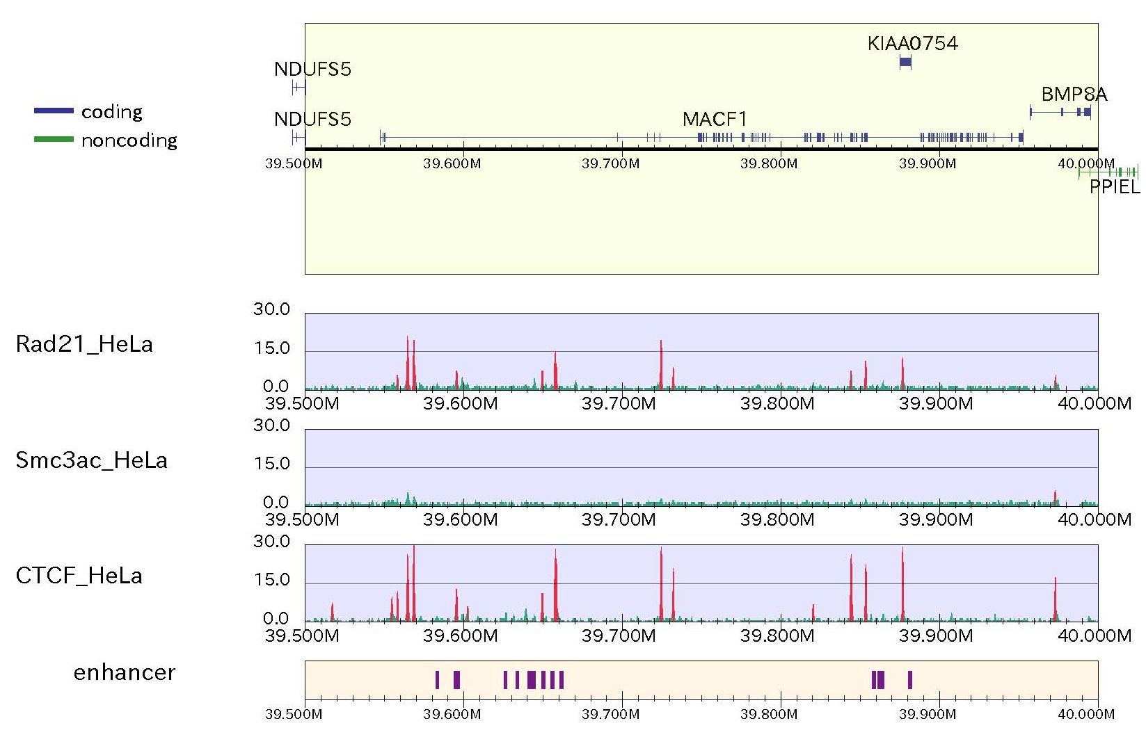
To identify broadly enriched region, use larger bin size (e.g., 1-kbp bin) and modified parameter set, e.g. as follows:
  % drompa2 PEAKCALL_P -p ChIPseq_broad-hg19 -gt genome_table-hg19.txt $s1 $s2 $s3 $s4 -g_ref refFlat_hg19.txt \
  % -optype2 -LS2000 -bs1 10 -bs2 10 -bs3 1000 -bs4 1000 -sm 2000 -ethre 2.0
Figure sample 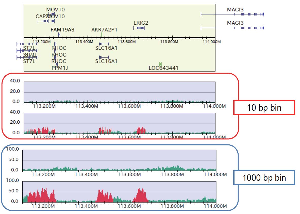
Enrichment test
For the small genome such as yeast, due to enough sequencing depth (>10 fold), the statistical reliability at every genomic position is large in each case.Therefore the genome-wide ChIP/Input enrichment distribution is also informative, which reflects the actual protein-binding probability at every position in the genome.
Options (for enrichment test)
     -ethre: first threshold of IP/Input enrichment
     -ethre2: second threshold of IP/Input enrichment
     -localmax: search localmax of IP/Input enrichment
     -localthre: threshold of IP/Input enrichment summit for -localmax option
     -lt: -localthre for st sample
     -ipm: read intensity threshold of peak summit
PEAKCALL_E command has the second threshold for ChIP/Input enrichment "-ethre2".
The enrichment distribution is highlighted in red, orange and gray.
Examples
To make a pdf file of the enrichment distribution map for yeast, type:% drompa2 PEAKCALL_E -p ChIPseq_yeast -gt genome_table_scer $s1 $s2 $s3 $s4 -showars -ars ARS-oriDB.txt \ % -optype2 -LPP2 -scale_ratio 1 -bn 3 -ystep 14 -ethre 1.5 -ethre2 1.2 -LS500 -rmchr
Figure sample 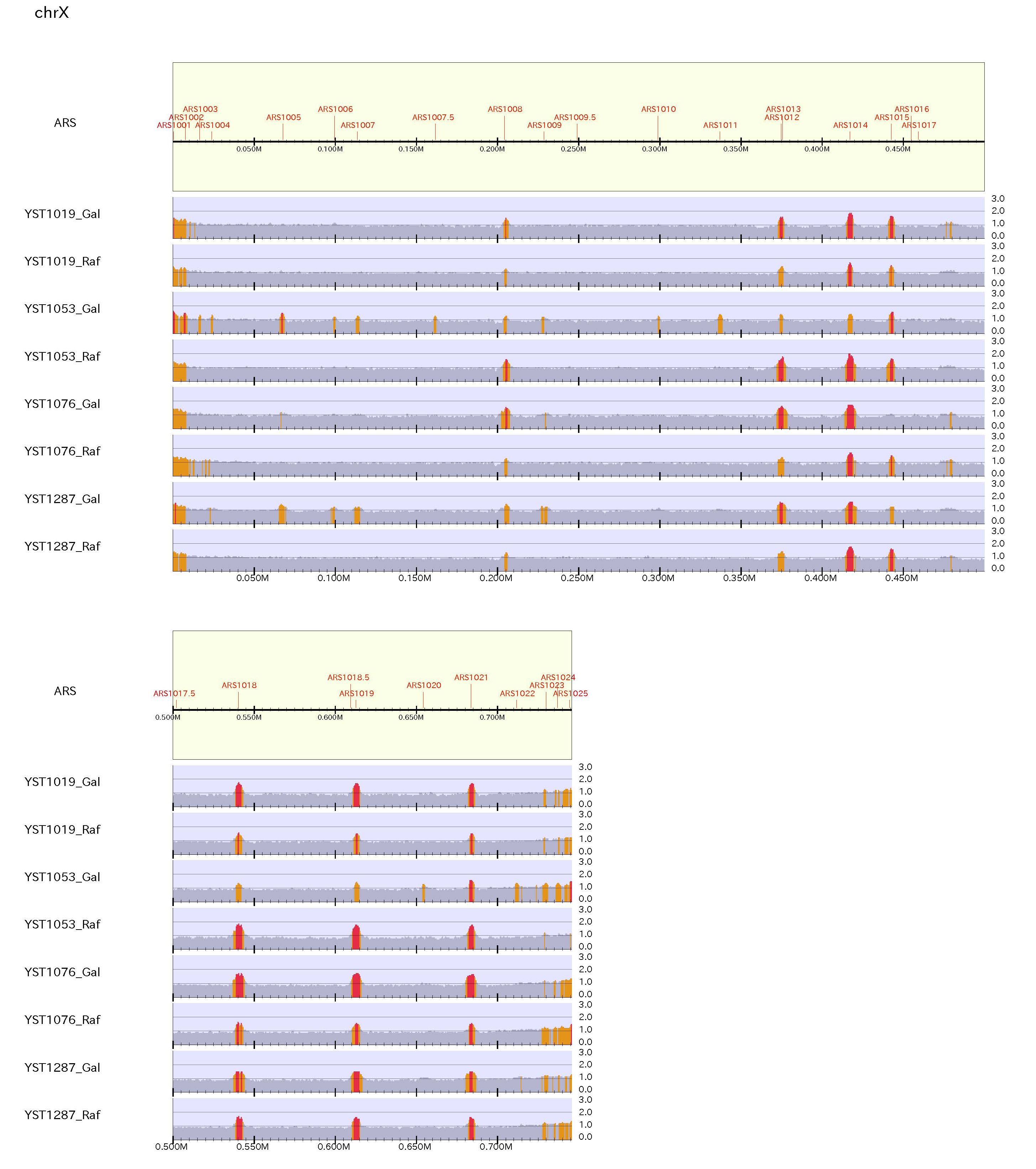
This figure shows the division of reads between after and before DNA replication for yeast. "-showars" option shows the ARS in the genome.
When supply "-ethre 1.5 -ethre2 1.2", the enrichment > 1.5 is highlighted in red while the enrichment from 1.2 to 1.5 is highlighted in orange.
It is possible to change the scale of each ratio line (y-axis) with "-scale_ratio" or "-scr" option. If you want to use logratio, supply "-showratio2".
If you want to output the genome-wide enrichment distribution the as wig file. use "-optype4" option.
% drompa2 PEAKCALL_E -nosig -p ChIPseq_yeast -gt genome_table_scer $s1 -optype4
localmax
"-localmax" option lines the peak summit which is over the enrichment threshold specified by "-localthre" or "-lt" option.When the highlight is not necessary, supply "-nosig" option.
  % drompa2 PEAKCALL_E -p localmax -gt genome_table_scer $s1 $s2 $s3 $s4 -localmax -localthre 1.5 -showars -ars ARS-oriDB.txt \
  % -optype2 -LPP2 -scale_ratio 1 -bn 3 -ystep 14 -rmchr -LS500
Figure sample 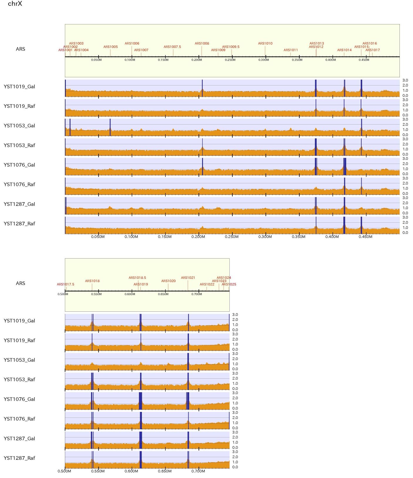
The neighboring localmax positions closer than 500 bp are merged into one position.
DROMPA: other functions
Global view
To make a chromosome-wide overview of the ChIP-seq data, specify command "GV":% drompa2 GV $s1 $s2 $s3 $s4 -p ChIPseq-wholegenome-hg19 -gt genome_table-hg19.txt \ % -graph GCcontents_hg19/ -gcsize 500000 -genedens gene_density_hg19/ -gdsize 500000
In this function, the default binsize is 100k-bp and ChIP/Input enrichment is shown.
When specifying "GV" command, DROMPA does not perform the significance test but simply highlight the bins containing ChIP/Input enrichments above the y axis (the value specified with option "-scale_ratio") in red.
Figure sample 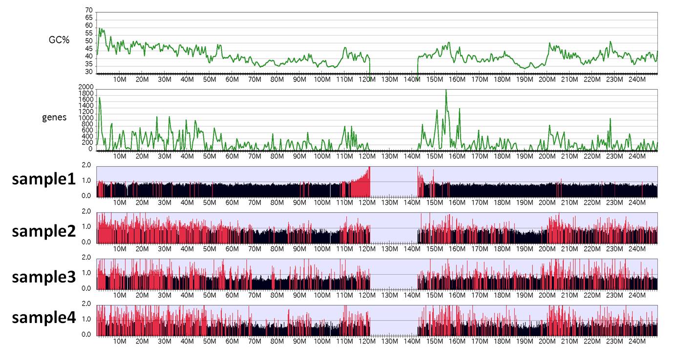
Peak density
PD command is to show the concentration of obtained peaks. This command requires "peakdensity.pl" in the scripts directory.To make the file which contains peak number with fixed length (here 500 kbp), type:
% peakdensity.pl ChIP1.xls ChIP1 500000 genome_table-hg19.txt
and apply PD command:
% drompa2 PD -p peakdensity -gt genome_table-hg19.txt -pd ChIP1 -pdname ChIP1 -pdsize 500000 -graph GCcontents_hg19/ -gcsize 500000
Figure sample 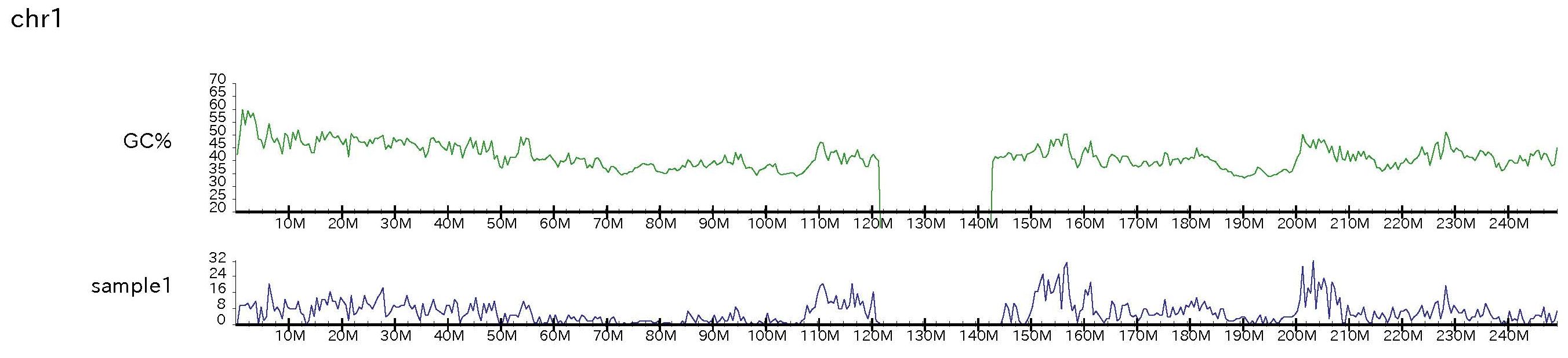
When the peak number is small, GOVERLOOK command is also useful.
% drompa2 GOVERLOOK -p overlook -gt genome_table-hg19.txt -bed peak1.bed -bedname peak1 -bed peak2.bed -bedname peak2
This command show the chromosome bar with the peaks specified by "-bed" option. GOVERLOOK command can treat up to three bed files.
Figure sample 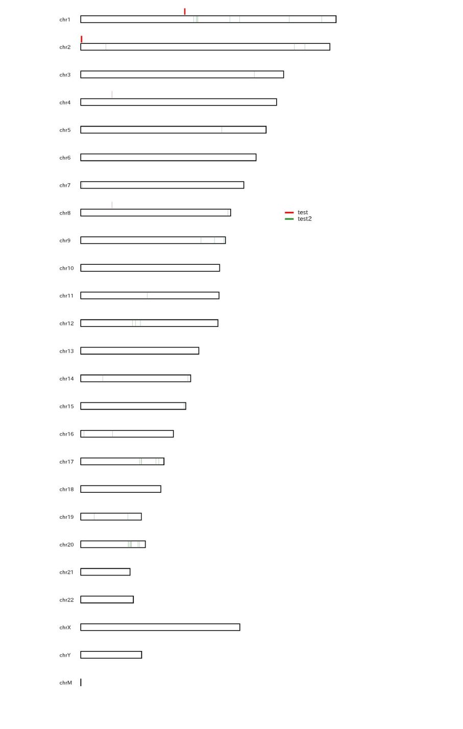
Count tag
COUNTTAG command outputs the accumulated read counts within the specified peak regions.Multiple samples can be applied at the same time.
drompa2 COUNTTAG -p counttag -gt genome_table-hg19.txt -i parse2wig2dir/CTCF -i parse2wig2dir/Rad21 -i parse2wig2dir/Input -peak peaks.xls
This score can be used to investigate FRiP (fraction of reads in peaks) [4] of each sample.
Compare intensity
CI command outputs the accumulated read number of each peaks specified by "-peak" options.This output can be used for the scatter plot of overlapped peak regions..
drompa2 CI -p counttag -gt genome_table-hg19.txt -i parse2wig2dir/CTCF -i parse2wig2dir/Rad21 -peak peaks.xls
Read distribution profile (require R)
DROMPA can show the averaged reads distribution around transcription start sites (TSS), transcription termination sites (TTS), gene bodies and specified peak list by supplying PROFILE command. Supply "-ptype" option to choose the profile type.For instance, to show read density around gene bodies, type as follows:
% drompa2 PROFILE -ptype3 -g_ref refFlat_hg19.txt $s1 $s2 $s3 $s4 -p aroundgene -gt genome_table-hg19.txt
Then DROMPA outputs a script for R. Do the R command:
% R --vanilla üā aroundgene.R
Then the pdf file "aroundgene.pdf" is output.
Figure sample 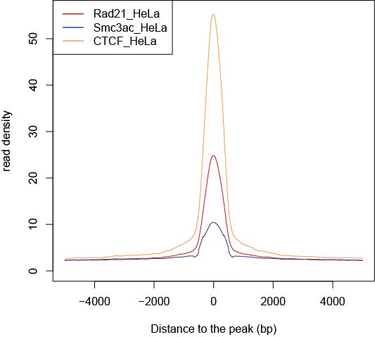
Normalization (option "-ntype")
In default, PROFILE command uses total read normalization (same as other commands). If you want to normalize reads with total mapped reads within target regions only, supply "-ntype1" option.Heatmap
From version 2.1.0, DROMPA can make heatmap pdf file of target sites. Most options are similar to those for PROFILE command.Options (for HEATMAP)
     -ptype: (1; around TSS, 2; around TES, 3; divide gene into 100 subregions 4; around peak sites)
     -stype: (0; read 1; enrich 2; pvalue)
     -binsize: bin size (default: 100)
     -bed (-bedname): target regions (and name)
     -cw: width from the center (default: 2.5kb)
     -scale_tag: maxvalue for -stype0
     -scale_ratio: maxvalue for -stype1
     -scale_pvalue: maxvalue for -stype2
For instance, to show read density around TSSs, type as follows:
  % drompa2 HEATMAP -p heatmap -gt genome_table-hg19.txt $s1 $s2 $s3 $s4 \
  % -bed sites1.bed -bedname sites1 -bed sites2.bed -bedname sites2 -ptype4 -stype1
Figure sample 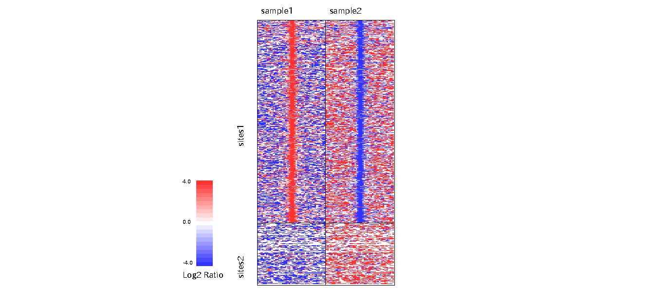
"-stype1" means "show ChIP/Input enrichment". "-scale_tag", "-scale_ratio" and "-scale_pvalue" define the max value of the color.
Mappability file
Since the mappability score depends on the genome, mapping tool and mapping parameter, it is necessary to make the mappability file for your analysis setting.While several mappability files can be downloaded from our websites, it can be made by our scripts.
Note: This procedure takes much computational resource and disk-space.
- Make the read file that contains k-mer reads generated from all possible positions of the genome with "make_kmers.pl"
- Map the read file onto the genome by the mapping tool with same setting for ChIP-seq analysis. For example,
- The program "cnt_mappability" converts mapfile to base-level mappability file in "mpbldir":
% cnt_mappability -i genome-50-n2-m1.bowtie -o genome-50-n2-m1 -gt genome_table-hg19.txt
- "convertmpbl2window.pl" script converts base-level mappability to window-level mappability:
% make_kmers.pl genome 50 > genome-50.fasta
% bowtie -f index genome-50.fasta -n2 -m1 -p12 --suppress 5 --suppress 6 > genome-50-n2-m1.bowtie
% convertmpbl2window.pl mpbldir/genome-50-n2-m1 genome_table-hg19.txt 1000
References
- Deardorff M.A., Bando M, Nakato, R. et al.: HDAC8 mutations in Cornelia de Lange syndrome affect the cohesin acetylation cycle. Nature, 2012.
- Nakato, R., Itoh T. and Shirahige K.: DROMPA: easy-to-handle peak calling and visualization software for the computational analysis and validation of ChIP-seq data, Genes to Cells, vol.18, issue 7, 2013.
- Kun Liang and Sunduz Keles: Normalization of ChIP-seq data with control. BMC Bioinformatics, 2012.
- Landt, S. G. et al. ChIP-seq guidelines and practices of the ENCODE and modENCODE consortia. Genome Research, 2012.
Ryuichiro Nakato (rnakato AT iam.u-tokyo.ac.jp)